Annotating regions of interest with napari

We will show:

1. how to use napari for drawing regions of interesets and how to access these annotations via code.

2. assuming these saved regions are anatomical regions of interterest, how to extract the Visium spots/cells under these regions.

For the sake of generality, instead of annotating the untransformed data, we will assign an affine transformation to the data and show that annotations and query APIs work in any coordinate system.

%load_ext jupyter_black

import numpy as np
import pandas as pd
import spatialdata as sd
from geopandas import GeoDataFrame
from shapely import Polygon
from spatialdata.models import ShapesModel
from spatialdata.transformations import Identity

import spatialdata_plot  # noqa: F401

# from napari_spatialdata import Interactive

Please download visium_associated_xenium_io data from https://spatialdata.scverse.org/en/stable/tutorials/notebooks/datasets/README.html. We will align the file, as shown in this analysis notebook.

Please rename the file to visium.zarr and place it in the same folder as this notebook (or use symlinks to make the data accessible).

Information regarding data licensing and attribution for the dataset listed above is available at: https://github.com/scverse/spatialdata-notebooks/tree/main/datasets.

visium_sdata = sd.read_zarr("visium.zarr")

visium_sdata

SpatialData object, with associated Zarr store: /Users/macbook/embl/projects/basel/spatialdata-data-converter/dependencies/spatialdata-sandbox/visium_associated_xenium_io/data.zarr
├── Images
│     ├── 'CytAssist_FFPE_Human_Breast_Cancer_full_image': DataTree[cyx] (3, 21571, 19505), (3, 10785, 9752), (3, 5392, 4876), (3, 2696, 2438), (3, 1348, 1219)
│     ├── 'CytAssist_FFPE_Human_Breast_Cancer_hires_image': DataArray[cyx] (3, 2000, 1809)
│     └── 'CytAssist_FFPE_Human_Breast_Cancer_lowres_image': DataArray[cyx] (3, 600, 543)
├── Shapes
│     ├── 'CytAssist_FFPE_Human_Breast_Cancer': GeoDataFrame shape: (4992, 2) (2D shapes)
│     └── 'visium_landmarks': GeoDataFrame shape: (3, 2) (2D shapes)
└── Tables
      └── 'table': AnnData (4992, 18085)
with coordinate systems:
    ▸ 'CytAssist_FFPE_Human_Breast_Cancer', with elements:
        CytAssist_FFPE_Human_Breast_Cancer_full_image (Images), CytAssist_FFPE_Human_Breast_Cancer_hires_image (Images), CytAssist_FFPE_Human_Breast_Cancer_lowres_image (Images), CytAssist_FFPE_Human_Breast_Cancer (Shapes), visium_landmarks (Shapes)
    ▸ 'CytAssist_FFPE_Human_Breast_Cancer_downscaled_hires', with elements:
        CytAssist_FFPE_Human_Breast_Cancer_hires_image (Images), CytAssist_FFPE_Human_Breast_Cancer (Shapes)
    ▸ 'CytAssist_FFPE_Human_Breast_Cancer_downscaled_lowres', with elements:
        CytAssist_FFPE_Human_Breast_Cancer_lowres_image (Images), CytAssist_FFPE_Human_Breast_Cancer (Shapes)
    ▸ 'aligned', with elements:
        CytAssist_FFPE_Human_Breast_Cancer_full_image (Images)

visium_sdata["table"].var

	gene_ids	feature_types	genome
SAMD11	ENSG00000187634	Gene Expression	GRCh38
NOC2L	ENSG00000188976	Gene Expression	GRCh38
KLHL17	ENSG00000187961	Gene Expression	GRCh38
PLEKHN1	ENSG00000187583	Gene Expression	GRCh38
PERM1	ENSG00000187642	Gene Expression	GRCh38
...	...	...	...
MT-ND4L	ENSG00000212907	Gene Expression	GRCh38
MT-ND4	ENSG00000198886	Gene Expression	GRCh38
MT-ND5	ENSG00000198786	Gene Expression	GRCh38
MT-ND6	ENSG00000198695	Gene Expression	GRCh38
MT-CYB	ENSG00000198727	Gene Expression	GRCh38

18085 rows × 3 columns

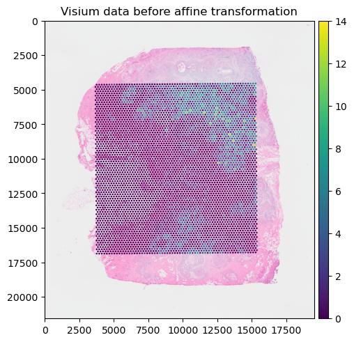
Let’s plot the data before adding an affine transformation to it.

(
    visium_sdata.pl.render_images("CytAssist_FFPE_Human_Breast_Cancer_full_image")
    .pl.render_shapes("CytAssist_FFPE_Human_Breast_Cancer", color="SAMD11")
    .pl.show(
        coordinate_systems="CytAssist_FFPE_Human_Breast_Cancer",
        title="Visium data before affine transformation",
    )
)

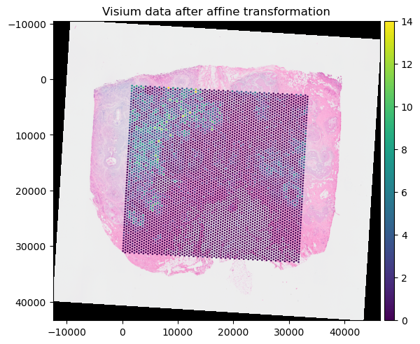
We use the same affine transformation derived in the “Alignemnt using landmarks” tutorial. For convenience, we will import the affine transformation and the postpone_transformation() function from a utils file.

from alignment_utils import AFFINE_VISIUM_XENIUM, postpone_transformation

print(AFFINE_VISIUM_XENIUM)

postpone_transformation(
    sdata=visium_sdata,
    transformation=AFFINE_VISIUM_XENIUM,
    source_coordinate_system="CytAssist_FFPE_Human_Breast_Cancer",
    target_coordinate_system="aligned",
)

Affine (x, y -> x, y)
    [ 1.61711846e-01  2.58258090e+00 -1.24575040e+04]
    [-2.58258090e+00  1.61711846e-01  3.98647301e+04]
    [0. 0. 1.]

(
    visium_sdata.pl.render_images("CytAssist_FFPE_Human_Breast_Cancer_full_image")
    .pl.render_shapes("CytAssist_FFPE_Human_Breast_Cancer", color="SAMD11")
    .pl.show(
        coordinate_systems="aligned",
        title="Visium data after affine transformation",
    )
)

Adding shapes annotations

We can use napari to draw rectangles and generic polygons.

This is the procedure to annotate and save the shapes (shown in the GIF):

1. open napari with Interactive() from napari_spatialdata

2. create a new Shapes layer in napari

3. (optional) rename the layer

4. (optional) change the fill and border propoerties for easier visualization

5. select the “Rectangle tool” or the “Polygon tool”

6. (optional) use the napari functions to move/delete/modify the shapes (shown later)

7. save the annotation to the SpatialData object by pressing Shift + E (if you called Interactive() passing multiple SpatialData objects, the annotations will be saved to one of them).

When pressing Shift + E, the shapes are saved. Anyway, for making this notebook reproducible, let’s manually hardcode the shapes that have been drawn in the GIF above. The code produces data that is equivalent to the one given by napari. Note that we could have also put the shapes in a new SpatialData objects, saved this to Zarr and loaded it here.

shape0 = np.array(
    [
        [7758.0, 11577.0, 11577.0, 7758.0, 7758.0],
        [10928.0, 10928.0, 17197.0, 17197.0, 10928.0],
    ]
)

shape1 = np.array(
    [
        [11721.0, 14712.0, 14712.0, 11721.0, 11721.0],
        [12117.0, 12117.0, 16801.0, 16801.0, 12117.0],
    ]
)
# fmt: off
shape2 = np.array(
    [
        [
            31320.0,28114.0,26745.0,26060.0,22998.0,23863.0,23899.0,29159.0,29195.0,32113.0,31789.0,33230.0,31320.0,
        ],
        [
            23286.0,20764.0,20836.0,19215.0,18170.0,15756.0,12081.0,12766.0,14567.0,17125.0,18530.0,20692.0,23286.0,
        ],
    ]
)
# fmt: on


def numpy_to_shapely(x: np.array) -> Polygon:
    return Polygon(list(map(tuple, x.T)))


gdf = GeoDataFrame(
    {
        "geometry": [
            numpy_to_shapely(shape0),
            numpy_to_shapely(shape1),
            numpy_to_shapely(shape2),
        ]
    }
)
gdf = ShapesModel.parse(gdf, transformations={"aligned": Identity()})
visium_sdata.shapes["my_shapes"] = gdf

Importantly, notice how the shapes "my_shapes", now available in the SpatialData object, are aligned to the "aligned" coordinate system. This is because the shapes have been drawn when the coordinate system "aligned" was selected in napari.

visium_sdata

SpatialData object, with associated Zarr store: /Users/macbook/embl/projects/basel/spatialdata-data-converter/dependencies/spatialdata-sandbox/visium_associated_xenium_io/data.zarr
├── Images
│     ├── 'CytAssist_FFPE_Human_Breast_Cancer_full_image': DataTree[cyx] (3, 21571, 19505), (3, 10785, 9752), (3, 5392, 4876), (3, 2696, 2438), (3, 1348, 1219)
│     ├── 'CytAssist_FFPE_Human_Breast_Cancer_hires_image': DataArray[cyx] (3, 2000, 1809)
│     └── 'CytAssist_FFPE_Human_Breast_Cancer_lowres_image': DataArray[cyx] (3, 600, 543)
├── Shapes
│     ├── 'CytAssist_FFPE_Human_Breast_Cancer': GeoDataFrame shape: (4992, 2) (2D shapes)
│     ├── 'my_shapes': GeoDataFrame shape: (3, 1) (2D shapes)
│     └── 'visium_landmarks': GeoDataFrame shape: (3, 2) (2D shapes)
└── Tables
      └── 'table': AnnData (4992, 18085)
with coordinate systems:
    ▸ 'CytAssist_FFPE_Human_Breast_Cancer', with elements:
        CytAssist_FFPE_Human_Breast_Cancer_full_image (Images), CytAssist_FFPE_Human_Breast_Cancer_hires_image (Images), CytAssist_FFPE_Human_Breast_Cancer_lowres_image (Images), CytAssist_FFPE_Human_Breast_Cancer (Shapes), visium_landmarks (Shapes)
    ▸ 'CytAssist_FFPE_Human_Breast_Cancer_downscaled_hires', with elements:
        CytAssist_FFPE_Human_Breast_Cancer_hires_image (Images), CytAssist_FFPE_Human_Breast_Cancer (Shapes)
    ▸ 'CytAssist_FFPE_Human_Breast_Cancer_downscaled_lowres', with elements:
        CytAssist_FFPE_Human_Breast_Cancer_lowres_image (Images), CytAssist_FFPE_Human_Breast_Cancer (Shapes)
    ▸ 'aligned', with elements:
        CytAssist_FFPE_Human_Breast_Cancer_full_image (Images), CytAssist_FFPE_Human_Breast_Cancer_hires_image (Images), CytAssist_FFPE_Human_Breast_Cancer_lowres_image (Images), CytAssist_FFPE_Human_Breast_Cancer (Shapes), my_shapes (Shapes), visium_landmarks (Shapes)
with the following elements not in the Zarr store:
    ▸ my_shapes (Shapes)

The shapes are stored in a geopandas.GeoDataFrame as shapely.Polygon objects. Hence we can use them in any geopandas/shapely workflow.

visium_sdata["my_shapes"]

	geometry
0	POLYGON ((7758 10928, 11577 10928, 11577 17197...
1	POLYGON ((11721 12117, 14712 12117, 14712 1680...
2	POLYGON ((31320 23286, 28114 20764, 26745 2083...

We can quickly see the shapes in the notebook (thanks to shapely). For more complex visualization involving different elements or different coordinate system we can rely on spatialdata-plot.

visium_sdata["my_shapes"].geometry.iloc[0]

visium_sdata["my_shapes"].geometry.iloc[2]

Manipulating the shapes in napari

Here is an example of how we can use napari to move/modify/delete some of the shapes, and save them to another layer (in-place overwrite is also supported).

Interactive(visium_sdata)

We saved the new layer as my_shapes_2 inside the same SpatialData object (again using the "aligned" coordinate system).

As above, let’s hardcode the shapes to make this notebook reproducible.

shape0 = np.array(
    [
        [3471.0, 7290.0, 7290.0, 3471.0, 3471.0],
        [5848.0, 5848.0, 12117.0, 12117.0, 5848.0],
    ]
)

shape1 = np.array(
    [
        [18278.0, 21269.0, 21269.0, 18278.0, 18278.0],
        [3435.0, 3435.0, 8118.0, 8118.0, 3435.0],
    ]
)

# fmt: off
shape2 = np.array(
    [
        [
            37049.0,28114.0,26745.0,26060.0,4696.0,23863.0,25160.0,29159.0,29195.0,32113.0,31789.0,33230.0,37049.0,
        ],
        [
            34274.0,20764.0,20836.0,19215.0,20116.0,15756.0,84.0,12766.0,14567.0,17125.0,18530.0,20692.0,34274.0,
        ],
    ]
)
# fmt: on

gdf = GeoDataFrame(
    {
        "geometry": [
            numpy_to_shapely(shape0),
            numpy_to_shapely(shape1),
            numpy_to_shapely(shape2),
        ]
    }
)
gdf = ShapesModel.parse(gdf, transformations={"aligned": Identity()})
visium_sdata.shapes["my_shapes_2"] = gdf

visium_sdata

SpatialData object, with associated Zarr store: /Users/macbook/embl/projects/basel/spatialdata-data-converter/dependencies/spatialdata-sandbox/visium_associated_xenium_io/data.zarr
├── Images
│     ├── 'CytAssist_FFPE_Human_Breast_Cancer_full_image': DataTree[cyx] (3, 21571, 19505), (3, 10785, 9752), (3, 5392, 4876), (3, 2696, 2438), (3, 1348, 1219)
│     ├── 'CytAssist_FFPE_Human_Breast_Cancer_hires_image': DataArray[cyx] (3, 2000, 1809)
│     └── 'CytAssist_FFPE_Human_Breast_Cancer_lowres_image': DataArray[cyx] (3, 600, 543)
├── Shapes
│     ├── 'CytAssist_FFPE_Human_Breast_Cancer': GeoDataFrame shape: (4992, 2) (2D shapes)
│     ├── 'my_shapes': GeoDataFrame shape: (3, 1) (2D shapes)
│     ├── 'my_shapes_2': GeoDataFrame shape: (3, 1) (2D shapes)
│     └── 'visium_landmarks': GeoDataFrame shape: (3, 2) (2D shapes)
└── Tables
      └── 'table': AnnData (4992, 18085)
with coordinate systems:
    ▸ 'CytAssist_FFPE_Human_Breast_Cancer', with elements:
        CytAssist_FFPE_Human_Breast_Cancer_full_image (Images), CytAssist_FFPE_Human_Breast_Cancer_hires_image (Images), CytAssist_FFPE_Human_Breast_Cancer_lowres_image (Images), CytAssist_FFPE_Human_Breast_Cancer (Shapes), visium_landmarks (Shapes)
    ▸ 'CytAssist_FFPE_Human_Breast_Cancer_downscaled_hires', with elements:
        CytAssist_FFPE_Human_Breast_Cancer_hires_image (Images), CytAssist_FFPE_Human_Breast_Cancer (Shapes)
    ▸ 'CytAssist_FFPE_Human_Breast_Cancer_downscaled_lowres', with elements:
        CytAssist_FFPE_Human_Breast_Cancer_lowres_image (Images), CytAssist_FFPE_Human_Breast_Cancer (Shapes)
    ▸ 'aligned', with elements:
        CytAssist_FFPE_Human_Breast_Cancer_full_image (Images), CytAssist_FFPE_Human_Breast_Cancer_hires_image (Images), CytAssist_FFPE_Human_Breast_Cancer_lowres_image (Images), CytAssist_FFPE_Human_Breast_Cancer (Shapes), my_shapes (Shapes), my_shapes_2 (Shapes), visium_landmarks (Shapes)
with the following elements not in the Zarr store:
    ▸ my_shapes (Shapes)
    ▸ my_shapes_2 (Shapes)

visium_sdata["my_shapes_2"].geometry.iloc[2]

Lasso annotations

We are working with the napari developers for enabling a lasso tool for drawing anatomical annotations. This functionality will be part of napari as a new button in the user interface. With SpatialData it will be possible to save and represent the annotatoins in-memory, as shown above. The lasso tool will have support for both mouse/trackpad and graphic tables.

In the GIF you can see a preview, the experimental code is available at https://github.com/napari/napari/pull/5555.

# we rounded the coordinates to make it less verbose here in the notebook
# fmt: off
shape0 = (
    np.array(
        [
            [
                182.0,181.0,179.0,178.0,174.0,173.0,172.0,168.0,165.0,164.0,164.0,166.0,167.0,168.0,169.0,169.0,168.0,166.0,163.0,163.0,
                163.0,164.0,165.0,167.0,168.0,169.0,172.0,173.0,174.0,175.0,180.0,185.0,187.0,188.0,189.0,190.0,191.0,192.0,193.0,194.0,
                196.0,198.0,200.0,202.0,205.0,207.0,209.0,211.0,212.0,213.0,215.0,215.0,216.0,216.0,215.0,215.0,214.0,212.0,211.0,209.0,
                208.0,208.0,206.0,205.0,204.0,202.0,200.0,196.0,195.0,195.0,195.0,194.0,192.0,190.0,189.0,186.0,184.0,184.0,183.0,184.0,
                185.0,186.0,186.0,184.0,182.0,182.0,182.0,183.0,183.0,183.0,182.0,182.0,183.0,183.0,181.0,178.0,178.0,178.0,179.0,180.0,
                182.0,182.0,183.0,183.0,182.0,
            ],
            [
                105.0,105.0,106.0,107.0,108.0,109.0,110.0,112.0,114.0,115.0,118.0,121.0,122.0,123.0,125.0,126.0,129.0,136.0,140.0,141.0,
                143.0,151.0,153.0,155.0,157.0,158.0,160.0,162.0,162.0,163.0,168.0,173.0,174.0,174.0,175.0,176.0,178.0,179.0,179.0,181.0,
                181.0,182.0,183.0,183.0,183.0,183.0,182.0,181.0,179.0,177.0,174.0,173.0,170.0,167.0,164.0,160.0,159.0,158.0,159.0,161.0,
                161.0,161.0,158.0,156.0,156.0,156.0,157.0,160.0,161.0,162.0,164.0,164.0,164.0,162.0,161.0,160.0,159.0,157.0,156.0,153.0,
                151.0,148.0,147.0,145.0,144.0,143.0,141.0,139.0,137.0,136.0,135.0,134.0,132.0,131.0,129.0,126.0,123.0,120.0,118.0,115.0,
                112.0,111.0,110.0,109.0,105.0,
            ],
        ]
    )
    * 100
)
# fmt: on

gdf = GeoDataFrame({"geometry": [numpy_to_shapely(shape0)]})
gdf = ShapesModel.parse(gdf, transformations={"aligned": Identity()})
visium_sdata.shapes["lasso"] = gdf

visium_sdata.shapes["lasso"].geometry.iloc[0]

(
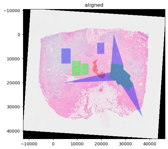
    visium_sdata.pl.render_images("CytAssist_FFPE_Human_Breast_Cancer_full_image")
    .pl.render_shapes("lasso", color="#ff000060")
    .pl.render_shapes("my_shapes", color="#00ff0060")
    .pl.render_shapes("my_shapes_2", color="#0000ff60")
    .pl.show(coordinate_systems="aligned")
)

INFO     Value for parameter 'color' appears to be a color, using it as such.                                      
INFO     Value for parameter 'color' appears to be a color, using it as such.                                      
INFO     Value for parameter 'color' appears to be a color, using it as such.

Extracting cells under the regions

Let’s now find the cells under each of the three regions of interest and record, in the table as a categorical column, which category each cell belongs. We will use the spatial query API polygon_query(); a separate tutorial is available for it and we will further assume the reader being familiar which such functionality.

Please note that, for how we constructed the shapes, some shapes overlap. In such case we will assign the labels of one of the categories (the one appearing last in our loop below).

Let’s find, for each saved shape, the table of cells it contains.

from spatialdata import polygon_query
import anndata as ad
from collections import defaultdict

filtered_tables_unmerged: dict[str, list[ad.AnnData]] = defaultdict(list)
filtered_tables: dict[str, ad.AnnData] = {}

for shape in ["lasso", "my_shapes", "my_shapes_2"]:
    for polygon in visium_sdata[shape].geometry:
        table = polygon_query(visium_sdata, polygon=polygon, target_coordinate_system="aligned")["table"]
        filtered_tables_unmerged[shape].append(table)
    filtered_tables[shape] = ad.concat(filtered_tables_unmerged[shape])

filtered_tables

{'lasso': AnnData object with n_obs × n_vars = 102 × 18085
     obs: 'in_tissue', 'array_row', 'array_col', 'spot_id', 'region'
     obsm: 'spatial',
 'my_shapes': AnnData object with n_obs × n_vars = 575 × 18085
     obs: 'in_tissue', 'array_row', 'array_col', 'spot_id', 'region'
     obsm: 'spatial',
 'my_shapes_2': AnnData object with n_obs × n_vars = 973 × 18085
     obs: 'in_tissue', 'array_row', 'array_col', 'spot_id', 'region'
     obsm: 'spatial'}

Note that polygon_query only returns a table in case of the table annotating an element in the resulting queried SpatialData object. Other tables are filtered out. Should you want to keep tables that are not annotating any elements in the resulting SpatialData object, a parameter filter_tables set to False can be passed on to the polygon_query function. Which region(s) or elements a table annotates can be retrieved as follows:

from spatialdata import SpatialData

# Note that we could also do visium_sdata.get_annotated regions here. This is just meant to show we
# can also get annotated regions from a table outside a Spatialdata object.
print(SpatialData.get_annotated_regions(visium_sdata["table"]))

['CytAssist_FFPE_Human_Breast_Cancer']

It can be that a table is annotating an element but is still not returned after the polygon query. The reason in that case is that the resulting table didn’t contain any rows annotating elements in the result of the query.

Now, let’s add a categorical column to the original full table, named 'annotation', with default categorical value 'unassigned'. Then, let’s assign, for each row in the 3 subtables, its value to the name of the relative region of interest.

# it's important for the index to be unique
assert visium_sdata["table"].obs.index.is_unique

categories = ["unassigned"] + list(filtered_tables.keys())
n = len(visium_sdata["table"])

visium_sdata["table"].obs["annotation"] = pd.Categorical(["unassigned" for _ in range(n)], categories=categories)

for shape, subtable in filtered_tables.items():
    in_shape = subtable.obs.index
    visium_sdata["table"].obs["annotation"].loc[in_shape] = shape

visium_sdata["table"].obs["annotation"].value_counts()

annotation
unassigned     3720
my_shapes_2     973
my_shapes       226
lasso            73
Name: count, dtype: int64

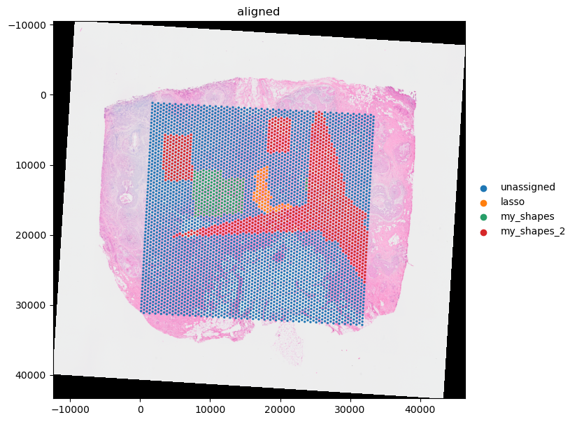
Let’s visualize the result.

import matplotlib.pyplot as plt

plt.figure(figsize=(12, 7))
ax = plt.gca()
(
    visium_sdata.pl.render_images("CytAssist_FFPE_Human_Breast_Cancer_full_image")
    .pl.render_shapes("CytAssist_FFPE_Human_Breast_Cancer", color="annotation")
    # .pl.render_shapes("lasso", color="#00000040")
    # .pl.render_shapes("my_shapes", color="#00000040")
    # .pl.render_shapes("my_shapes_2", color="#00000040")
    .pl.show(coordinate_systems="aligned", ax=ax)
)

Limitations

Currently we support saving rectangles, polygons and points with napari (see the landmark tutorial). We currently don’t support saving circles, ellipses or segments. Furthermore, we ignore the style parameters that napari provides, such us fill color, border color, points size and line width. If you are interested in saving these types of annotations please get in touch with us or join the NGFF discussions on annotations in GitHub.