Technology focus: 10x Genomics Visium#
This notebook will present a rough overview of the plotting functionalities that spatialdata implements for Visium data.
Please download the visium data from https://spatialdata.scverse.org/en/stable/tutorials/notebooks/datasets/README.html and rename it (eventually using symlinks) to visium_brain.zarr.
Information regarding data licensing and attribution for the dataset listed above is available at: https://github.com/scverse/spatialdata-notebooks/tree/main/datasets.
visium_zarr_path = "./visium_brain.zarr"
import spatialdata as sd
import spatialdata_plot  # noqa: F401

visium_sdata = sd.read_zarr(visium_zarr_path)
visium_sdata
SpatialData object, with associated Zarr store: /Users/macbook/embl/projects/basel/spatialdata-integration-testing/dependencies/spatialdata-sandbox/visium/data.zarr
├── Images
│     ├── 'ST8059048_hires_image': DataArray[cyx] (3, 2000, 1969)
│     ├── 'ST8059048_lowres_image': DataArray[cyx] (3, 600, 591)
│     ├── 'ST8059050_hires_image': DataArray[cyx] (3, 2000, 1968)
│     └── 'ST8059050_lowres_image': DataArray[cyx] (3, 600, 590)
├── Shapes
│     ├── 'ST8059048': GeoDataFrame shape: (2987, 2) (2D shapes)
│     └── 'ST8059050': GeoDataFrame shape: (3497, 2) (2D shapes)
└── Tables
      └── 'table': AnnData (6484, 31053)
with coordinate systems:
    ▸ 'ST8059048', with elements:
        ST8059048_hires_image (Images), ST8059048 (Shapes)
    ▸ 'ST8059048_downscaled_lowres', with elements:
        ST8059048_lowres_image (Images), ST8059048 (Shapes)
    ▸ 'ST8059050', with elements:
        ST8059050_hires_image (Images), ST8059050 (Shapes)
    ▸ 'ST8059050_downscaled_lowres', with elements:
        ST8059050_lowres_image (Images), ST8059050 (Shapes)
Visualise the data#
We’re going to create a naiive visualisation of the data, overlaying the Visium spots and the tissue images. For this, we need to load the spatialdata_plot library which extends the sd.SpatialData object with the .pl module.
visium_sdata.pl.render_images().pl.render_shapes().pl.show("ST8059050")
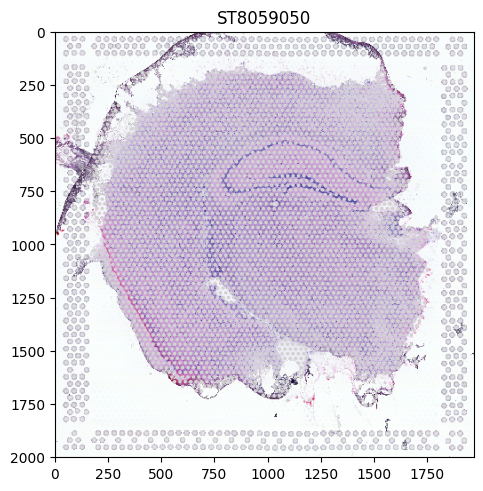
We can see that the data contains two coordinate systems (ST8059050 and ST8059052) with image and spot information each. In SpatialData, these spots are represented as Shapes. When giving no further parameters, one panel is generated per coordinate system with the members that have been specified in the function call. We can see that the spots are aligned to the tissue representation which is also respected by the plotting logic.
However, the spots are all grey since we have not provided any information on what they should encode. Such information can be found in the Table attribute (which is an anndata.AnnData table) of the SpatialData object, either in the data itself or the obs attribute.
visium_sdata["table"].to_df().sum(axis=0).sort_values(ascending=False).head(10)
# We will select some of the highly expressed genes for this example
mt-Co3     3292649.0
mt-Co1     3061428.0
mt-Atp6    2124067.0
mt-Co2     2110283.0
mt-Cytb    1288126.0
mt-Nd4     1073436.0
mt-Nd1     1073275.0
Ttr         832128.0
Fth1        828627.0
mt-Nd2      755237.0
dtype: float32
visium_sdata["table"].obs.head(3)
| in_tissue | array_row | array_col | spot_id | region | |
|---|---|---|---|---|---|
| AAACAAGTATCTCCCA-1 | 1 | 50 | 102 | 0 | ST8059048 |
| AAACACCAATAACTGC-1 | 1 | 59 | 19 | 1 | ST8059048 |
| AAACAGAGCGACTCCT-1 | 1 | 14 | 94 | 2 | ST8059048 |
Color the visium spots by gene expression#
To use this information in our plot, we pass the name of the column by which we want to color our expression to color. Furthermore, we are going to subset the data to only one coordinate system.
(
    visium_sdata.pl.render_images(elements="ST8059050_hires_image")
    .pl.render_shapes(elements="ST8059050", color="mt-Co3")
    .pl.show()
)
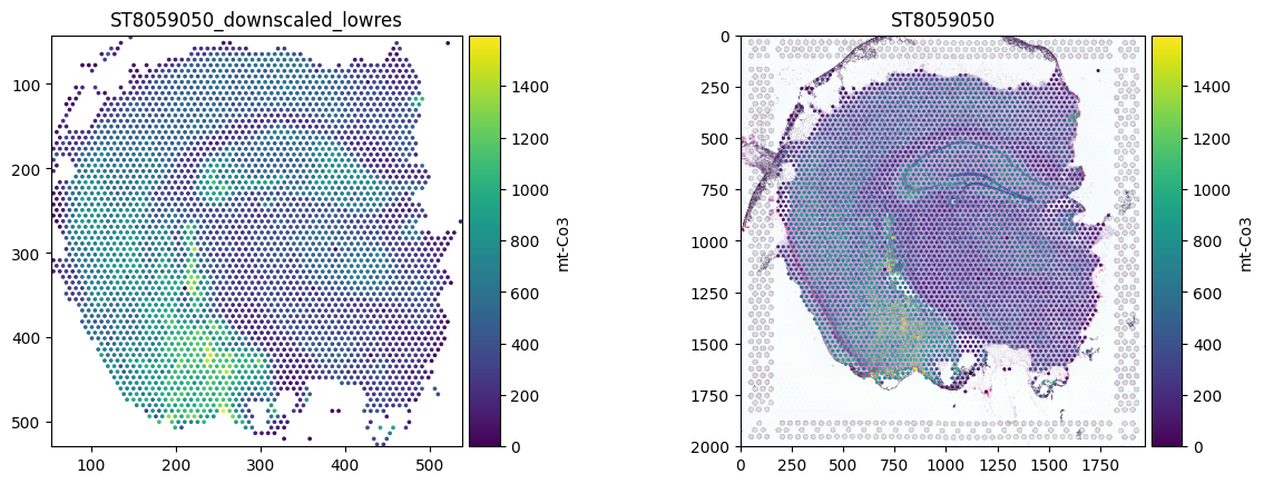
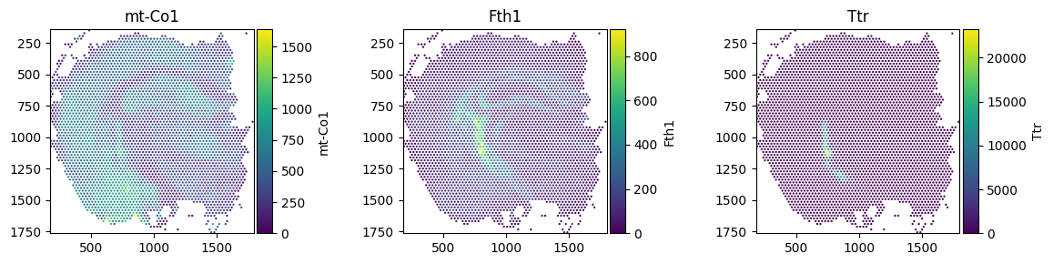
We can also provide ax objects to spatialdata_plot for further customisation.
import matplotlib.pyplot as plt

fig, axs = plt.subplots(ncols=3, nrows=1, figsize=(12, 3))

visium_sdata.pl.render_shapes(elements="ST8059050", color="mt-Co1").pl.show(ax=axs[0], title="mt-Co1", coordinate_systems="ST8059050")

visium_sdata.pl.render_shapes(elements="ST8059050", color="Fth1").pl.show(ax=axs[1], title="Fth1", coordinate_systems="ST8059050")

visium_sdata.pl.render_shapes(elements="ST8059050", color="Ttr").pl.show(ax=axs[2], title="Ttr", coordinate_systems="ST8059050")

plt.tight_layout()
For reproducibility#
# fmt: off

%load_ext watermark
# fmt: on
%watermark -v -m -p timeit,warnings,dask,datashader,matplotlib,numpy,pandas,scanpy,spatialdata,spatialdata_plot,geopandas,shapely
Python implementation: CPython
Python version       : 3.13.0
IPython version      : 9.15.0

timeit          : unknown
warnings        : unknown
dask            : 2026.6.0
datashader      : 0.19.1
matplotlib      : 3.10.9
numpy           : 2.4.6
pandas          : 2.3.3
scanpy          : 1.12.2
spatialdata     : 0.7.4.dev20+g0b9015b0e
spatialdata_plot: 0.4.1.dev39+g227434d0e
geopandas       : 1.1.4
shapely         : 2.1.2

Compiler    : Clang 18.1.8
OS          : Darwin
Release     : 25.5.0
Machine     : arm64
Processor   : arm
CPU cores   : 14
Architecture: 64bit