Technology focus: MERFISH#
This notebook will present a rough overview of the plotting functionalities that spatialdata implements for MERFISH data.
Please download the merfish data from https://spatialdata.scverse.org/en/stable/tutorials/notebooks/datasets/README.html and adjust the variable containing the location of the .zarr file.
Information regarding data licensing and attribution for the dataset listed above is available at: https://github.com/scverse/spatialdata-notebooks/tree/main/datasets.
merfish_zarr_path = "./merfish.zarr"
import spatialdata as sd
import spatialdata_plot  # noqa: F401

merfish_sdata = sd.read_zarr(merfish_zarr_path)
merfish_sdata
SpatialData object, with associated Zarr store: /Users/macbook/embl/projects/basel/spatialdata-sandbox/merfish/data.zarr
├── Images
│     └── 'rasterized': DataArray[cyx] (1, 522, 575)
├── Points
│     └── 'single_molecule': DataFrame with shape: (3714642, 3) (2D points)
├── Shapes
│     ├── 'anatomical': GeoDataFrame shape: (6, 1) (2D shapes)
│     └── 'cells': GeoDataFrame shape: (2389, 2) (2D shapes)
└── Tables
      └── 'table': AnnData (2389, 268)
with coordinate systems:
    ▸ 'global', with elements:
        rasterized (Images), single_molecule (Points), anatomical (Shapes), cells (Shapes)
Visualise the data#
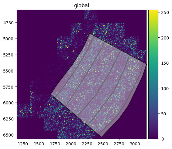
We’re going to create a naiive visualisation of the data, overlaying the annotated anatomical regions contained in anatomical and the tissue image. For this, we need to load the spatialdata_plot library which extends the sd.SpatialData object with the .pl module. Furthermore, we will only select the elements we want to plot using pp.get_elements().
merfish_sdata.subset(["anatomical", "rasterized"]).pl.render_images().pl.render_shapes(
    fill_alpha=0.5,
    outline_alpha=1.0,
).pl.show()
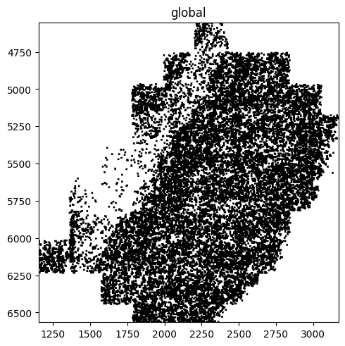
The MERFISH data also contains points which we have so far not visualised. This can be done with the pl.render_points() function. However, since we have over 3 million points, we will only render 1 % of them as to not overplot the image.
sampled_points = merfish_sdata.points["single_molecule"].sample(frac=0.01)
# fix attrs (see https://github.com/scverse/spatialdata/issues/1035)
sampled_points.attrs = merfish_sdata.points["single_molecule"].attrs
merfish_sdata.points["single_molecule"] = sampled_points
merfish_sdata.pl.render_points(color="black").pl.show()
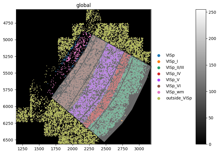
Furthermore, we can overlay all 3 layers and color the points by an annotation.
import matplotlib.pyplot as plt

fig, ax = plt.subplots(ncols=1, figsize=(6, 6))

(
    merfish_sdata.subset(["anatomical", "rasterized", "single_molecule"])
    .pl.render_images(cmap="gray")
    .pl.render_points(color="cell_type", size=1)
    .pl.render_shapes(fill_alpha=0.5, outline_alpha=1.0)
    .pl.show(ax=ax)
)